Machine Learning Methods for Causal Inference

Sean Ryder, December 11, 2020

The ability to anticipate the effect that a variable has on an outcome is a skill that is universally useful. Whether the problem is in business, politics, health, or everyday life, being able to estimate the effect of an input on conditional outcomes can lead to more efficient investment of resources. Modern advancements in big data collection and machine learning methods have made it possible to do just this. Recent machine learning methods for causal inference have recently arisen that have shown potential in real-world application. Many of these methods are built upon time-tested econometric models that can now be streamlined and iterated with machine learning. In this post, I describe two of the leading machine learning techniques for causal inference and their real-world applications.

Causal inference is a very different concept than prediction. The best example that I found for explaining the difference between prediction and causal inference is given by Kleinberg et al. as follows: Assume one individual is faced with a decision to invest in a rain dance in order to produce rain to water their crops. Assume a second individual is faced with a decision to bring an umbrella to work in case it rains. The first individual is interested in the causal effect of rain dances on the outcome of rain while the second individual is only interested in predicting the outcome of rain. There may also be certain instances when both causality and prediction are points of interest, as is the case in many counterfactual inference problems.

One of the hardest states of the world to examine is that of the counterfactual: a state of the world other than the current reality. This can include estimation of a previous outcome that was never realized, or the effect of a policy when a study is impossible to perform. Causal and counterfactual inference are closely related concepts. Both kinds of inference concern the causal effect of variables on outcomes. They differ in that counterfactual inference examines states of the world that have not been realized. An example of a counterfactual statement concerned with a past outcome would be “If the Covid-19 pandemic did not occur, then the current national GDP would be x.” Regardless of the type of modeling that is being done, the final goal is to create a model that can accurately predict future or counterfactual outcomes and causal effects based on test data.

One of the traditional methods for creating causal models has been the randomized control trial (RCT). This method involves conducting a study to gather data from randomized groups, one of which receives a treatment and another that is the control group. The data can then be modeled to estimate the treatment effect. Famous examples of RCT’s are the RAND and the Oregon Health Insurance Experiments; information on both of these can be found here and here, respectively. To briefly summarize the RAND health insurance experiment, facilitators were interested in the effect that cost sharing had on the utilization of insurance and health outcomes. Thousands of families were observed during this study that were all given different levels of price for insurance. The causal effect of these prices on insurance utilization and health outcomes was then calculated after observations had been collected from 1971-1982.

Although RCT’s have been useful in the past, conducting one may be impossible because of a number of circumstances. Excessive costs are sometimes needed to run experiments, as can be seen in the RAND experiment that cost over $300 million to run. Other than the immediate cost of conducting experiments, there may also be long term costs associated with the consumer’s attitude toward the firm(s) involved.

Utilizing the Deep IV Package for Counterfactual Inference

Employing instrumental variables is useful when controlled experiments are expensive or unobtainable for other reasons. Instrumental variables are variables that are independent from outcomes but have a causal relationship with another endogenous variable in the model. Endogenous variables would not be useful for modeling causal relationships as they are associated with both outcomes and the error term. An example of these variables given by the authors of the Deep IV package, that I will explain more later in this section, are the variables fuel costs and ticket price in relation to airline ticket sales. In this case, fuel costs would be the instrument as it is assumed to have a causal effect on ticket prices but not ticket sales. Ticket price, on the other hand, is an endogenous variable that has an effect on sales, which without modeling is an unquantified causal effect. The figure below illustrates how instrumental variables are related to the models they are concerned with. A more in-depth definition of an instrumental variable can be found here.

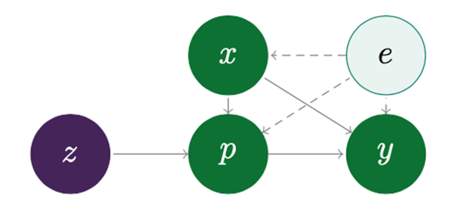
x = observable features, p = treatment variable, z = instruments, e = latent effects/error, y = outcome (Hartford et al.)

Deep IV is a machine learning package developed by Hartford et al. that leverages the use of instrumental variables to model causal relationships in the absence of experiments. Deep IV is a Python package that is a subclass of the Keras model, which is an API of the machine learning platform TensorFlow2.0. (Information about Keras and TensorFlow can be found here and here, respectively.) The Deep IV package works by using stochastic gradient descent to train a deep neural network of two stages. The first stage is the treatment network that finds the distribution of the treatment variable based on the observable covariates and the instrument. The second stage is the outcome network that finds the counterfactual function to model test data. Utilizing stochastic gradient descent to train this deep neural net entails minimizing a predetermined loss function based on the training data. After performing iterations of the minimized loss function, the final model is then validated on held-out data from the training data. The Deep IV package is available on GitHub here.

Applications for the Deep IV package exist mostly on a microeconomic scale. Modeling causal demand for airline tickets based on price is one example that the authors give for the use of their framework. An airline seeking to find the causal effect of prices on sales would most likely suffer extensive immediate and long term costs if it were to conduct a RCT on its customers. A naïve analysis of this relationship would also reveal that higher prices lead to more sales, which is obviously not the case, because of observable variables like volume of travelers over the holidays. It is for these reasons that instrumental variables must be implemented to realize the counterfactual causal relationship between price and sales. The instrument in this example, as previously mentioned, is given as fuel prices. While fuel prices are related to the price of a ticket, it is a variable that is independent of the outcome, sales, and the latent effects of the model. In this way, fuel costs can be passed through the Deep IV method as the instrument, z, in order to find the causal relationship between ticket prices and sales.

Generalized Random Forests for Causal Inference

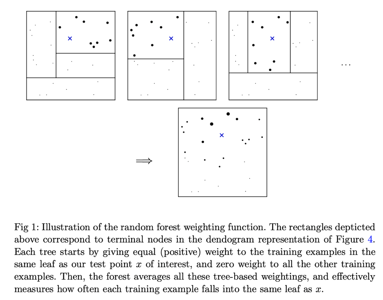
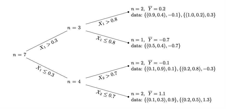
Random forest is a machine learning method that has been around for quite some time and has seen success in many real-world applications. The primary function of random forests has been solely on estimating expected outcomes. Generalized random forest (GRF) is a related method more recently developed that goes beyond the functionality of traditional random forests as a means to model “…non-parametric quantile regression, conditional average partial effect estimation, and heterogeneous treatment effect estimation via instrumental variables” (Athey et al. 2018). Measurement of split quality is one factor that differentiates GRF from traditional random forests. Split quality is determined by the best variables on which to split a node into within a decision tree. While the split quality being measured is dependent upon the type of modeling being done, the overall quality is based on the heterogeneity of child node. This means that GRF maximizes the difference in treatment effect among two child nodes when performing a split. Another process that defines GRF training is weighting of similar leaves in the forest. Susan Athey explained in a presentation at the 2018 Conference on Neural Information Processing Systems that in GRF, neighborhood functions are generated to locally analyze the treatment effect on a variable with other covariates in the “neighborhood,” or closer in the forest, weighted more heavily than those that are farther from the variable in question. GRF also incorporates a feature called “honest estimation” that divides the training data into two subsets: one that partitions the forest and one that assigns weights to the leaves. The GRF package for R can be found on GitHub here. Seen below are diagrams of the forest weighting function (and the description given by Athey et al. 2018) and an example of a resulting dendrogram.

Included in the GRF package is a function titled “causal forest.” This function is used to estimate the heterogeneous treatment effect of a binary variable on outcomes. The function starts by using the framework defined in the broader GRF package that was previously described. Causal forest then utilizes two measures during modeling to insure a more accurate estimation of the treatment effect. The first measure, orthogonalization, is used to limit the trivial effect of propensity scores that may lead to useless splits in the forest. A propensity score is the probability that a subject receives treatment based on its observed characteristics. Further information on propensity scores and how they are used can be found here. Orthogonalization first estimates propensity scores and marginal outcomes by training separate forests and obtaining an out-of-bag estimate. These estimates are then used to compute the residual treatment and outcome. The final forest is then trained on these residuals. The second measure taken by causal forest deals with balancing the size of child nodes as well as the number of control and treated examples. This is done by defining a minimum node size within the function as well as an imbalance penalty for nodes that contain too many of either control or treated examples.

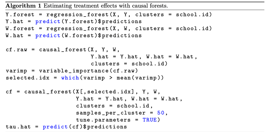
The creators of this method utilized causal forest on a simulated dataset from the National Study of Learning Mindsets to find the effect of some binary treatment variable W on learning-achievement outcomes. The treatment variable is described as “…a nudge-like intervention designed to instill students with a growth mindset on student achievement” (Athey et al. 2019). A number of other variables were included in the model, a list of which can be seen below:

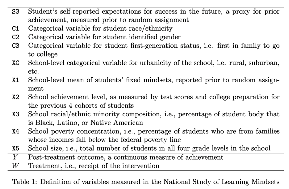
The final forest that was used to model the data was trained in two stages: the first was trained on all of the variables listed and the second was trained on only those variables that saw a substantial number of splits in the first stage. Using the average treatment effect function included in GRF, it was found that treatment had a large positive effect on outcomes. While there was no strong heterogeneity present when all variables were taken into account, when limited to X1 and X2 heterogeneity could be found in X1. X1 was one of the most important variables in the set and accounted for around 24% of splits in the forest. Below can be seen the algorithm that was used to predict the treatment effect:

Further Applications

The combination of machine learning methods and causal inference creates powerful tools for causal inference that have the ability to estimate counterfactual outcomes in order to make real-world decisions. Many applications of machine learning in both micro- and macroeconomic settings have yet to manifest themselves in the development of policy. Aside from the microeconomic policy example previously given with regards to airline ticket sales, I believe that similar modeling can be performed to anticipate the causal effect of macroeconomic policy on the broader economy. Fiscal and monetary policy are very complex areas of interest that have the potential to impact many areas of the macroeconomy. Eventually, machine learning methods similar to those I have presented in this post may be able to model the causal effect of policy on macroeconomic indicators and outcomes such as gross domestic product, unemployment rates, and disposable personal income, among others. I believe that the utilization of machine learning in causal inference will continue to grow at a fast rate in order to produce smarter, more effective policies.